Jason A. French

Northwestern University

Fixing Knitr: Formatting Statistical Output to 2 Digits in R

| Comments

Overview of reproducible research

Reproducible research is a phrase that describes an academic paper or manuscript that contains the code and data in addition to what is usually published - the researcher’s interpretation. In doing so, the experimental design and method of analysis is easily replicated by unaffiliated labs and critiqued by reviewers as the full analysis used to produce the results is submitted along with the final paper. One way of producing reproducible research is to use R code directly inside your LaTeX document. In order to faciliate the combination of statistical code and manuscript writing, two R packages in particular have arisen: Sweave and knitr. knitr is an R package designed as a replacement for Sweave, but both packages combine your R analysis with your LaTeX manuscript (i.e., knitr = R + LaTeX).

One advantage of knitr is that the researcher can easily create ANOVA and demographic tables directly from the data without messing around in Excel. However, as we’ll see, both knitr and Sweave can run into problems when formatting your table values to 2 decimal points. In this post, I’ll detail my proposed method of fixing that which can be applied to your entire mansucript by editing the beginning of your knitr preamble.

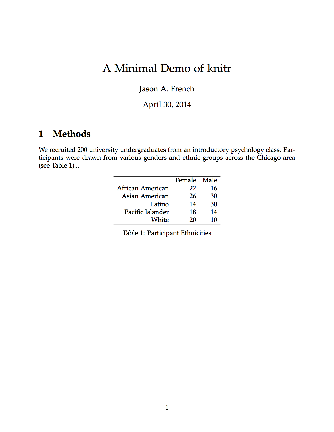
The basic example below contains the beginning of a hypothetical Methods section of a manuscript. We want to take the values from an R table, which has the breakdown of participants by gender and ethnicity, and display them as numbers in our manuscript.

Basic knitr.Rnw Example
1
2
3
4
5
6
7
8
9
10
11
12
13
14
15
16
17
18
19
20
21
22
23
24
25
26
27
28
29
30
31
32
33
34
35
36
37
38
39
40
41
42
43
44
45
46
47
48
\documentclass[12pt]{article}
\usepackage[sc]{mathpazo}
\usepackage[T1]{fontenc}
\usepackage{geometry}
\geometry{verbose,tmargin=2.5cm,bmargin=2.5cm,lmargin=2.5cm,rmargin=2.5cm}
\setcounter{secnumdepth}{2}
\setcounter{tocdepth}{2}
\usepackage{url}
\usepackage[unicode=true,pdfusetitle,
 bookmarks=true,bookmarksnumbered=true,bookmarksopen=true,bookmarksopenlevel=2,
 breaklinks=false,pdfborder={0 0 1},backref=false,colorlinks=false]
 {hyperref}
\hypersetup{
 pdfstartview={XYZ null null 1}}
\usepackage{breakurl}
\begin{document}

<<setup, include=FALSE, cache=FALSE>>=
library(knitr)
# set global chunk options
opts_chunk$set(fig.path='figure/minimal-', fig.align='center', fig.show='hold')
options(replace.assign=TRUE,width=90)
@

\title{A Minimal Demo of knitr}
\author{Jason A. French}
\maketitle


<<random-ethnicity, include=FALSE>>=
# Create data.frame of random ethnicities
x <- data.frame(Ethnicity = sample(as.factor(
  rep(x = c('White','African American','Asian American', 'Latino', 'Pacific Islander')
    )
  ),size = 100, replace = TRUE),
  Gender=rep(c('Male', 'Female'),100))
x.table <- table(x)
@

\section{Methods}
We recruited \Sexpr{sum(x.table)} university undergraduates from an introductory psychology class. Participants were drawn from various genders and ethnic groups across the Chicago area (see Table~\ref{tab:ethnicity})...

<<ethnicity-table, echo = FALSE, results = 'asis'>>=
library(xtable)
xtable(x.table, caption = 'Participant Ethnicities', label='tab:ethnicity')
@

\end{document}

As we see below, running the knit() command on our knitr manuscript inside R produces a regular LaTeX file that can be compiled with to a PDF using pdflatex or TeX Shop. Notice that the R table objects have been replaced with LaTeX tables.

Running knit() knitr.Rnw inside R
1
2
library(knitr)
knit(input = 'knitr.Rnw', output = 'knitr.tex')
Resulting knitr.tex LaTeX document
1
2
3
4
5
6
7
8
9
10
11
12
13
14
15
16
17
18
19
20
21
22
23
24
25
26
27
28
29
30
31
32
33
34
35
36
37
38
39
40
41
42
43
44
45
46
47
48
49
50
51
52
53
54
55
56
57
58
59
60
61
62
63
\documentclass[12pt]{article}\usepackage[]{graphicx}\usepackage[]{color}
\makeatletter
\definecolor{fgcolor}{rgb}{0.345, 0.345, 0.345}
\newcommand{\hlnum}[1]{\textcolor[rgb]{0.686,0.059,0.569}{#1}}
\newcommand{\hlstr}[1]{\textcolor[rgb]{0.192,0.494,0.8}{#1}}
\newcommand{\hlcom}[1]{\textcolor[rgb]{0.678,0.584,0.686}{\textit{#1}}}
\newcommand{\hlopt}[1]{\textcolor[rgb]{0,0,0}{#1}}
\newcommand{\hlstd}[1]{\textcolor[rgb]{0.345,0.345,0.345}{#1}}
\newcommand{\hlkwa}[1]{\textcolor[rgb]{0.161,0.373,0.58}{\textbf{#1}}}
\newcommand{\hlkwb}[1]{\textcolor[rgb]{0.69,0.353,0.396}{#1}}
\newcommand{\hlkwc}[1]{\textcolor[rgb]{0.333,0.667,0.333}{#1}}
\newcommand{\hlkwd}[1]{\textcolor[rgb]{0.737,0.353,0.396}{\textbf{#1}}}

\usepackage{framed}

\definecolor{shadecolor}{rgb}{.97, .97, .97}
\definecolor{messagecolor}{rgb}{0, 0, 0}
\definecolor{warningcolor}{rgb}{1, 0, 1}
\definecolor{errorcolor}{rgb}{1, 0, 0}
\newenvironment{knitrout}{}{} % an empty environment to be redefined in TeX

\usepackage{alltt}
\usepackage[sc]{mathpazo}
\usepackage[T1]{fontenc}
\usepackage{geometry}
\geometry{verbose,tmargin=2.5cm,bmargin=2.5cm,lmargin=2.5cm,rmargin=2.5cm}
\setcounter{secnumdepth}{2}
\setcounter{tocdepth}{2}
\usepackage{url}
\usepackage[unicode=true,pdfusetitle,
 bookmarks=true,bookmarksnumbered=true,bookmarksopen=true,bookmarksopenlevel=2,
 breaklinks=false,pdfborder={0 0 1},backref=false,colorlinks=false]
 {hyperref}
\hypersetup{
 pdfstartview={XYZ null null 1}}
\usepackage{breakurl}
\IfFileExists{upquote.sty}{\usepackage{upquote}}{}
\begin{document}

\title{A Minimal Demo of knitr}
\author{Jason A. French}
\maketitle

\section{Methods}
We recruited 200 university undergraduates from an introductory psychology class. Participants were drawn from various genders and ethnic groups across the Chicago area (see Table~\ref{tab:ethnicity})...

\begin{table}[ht]
\centering
\begin{tabular}{rrr}
\hline
 & Female & Male \\
\hline
African American &  22 &  16 \\
Asian American &  26 &  30 \\
Latino &  14 &  30 \\
Pacific Islander &  18 &  14 \\
White &  20 &  10 \\
\hline
\end{tabular}
\caption{Participant Ethnicities}
\label{tab:ethnicity}
\end{table}
\end{document}

Last, after compiling our LaTeX file using TeX Shop, we’re greeted with the final product below:

Summary thus far

The example above used data from R directly in a sentence in the Methods section (i.e., “We recruited 200 university undergraduates from an introductory psychology class.”) and did so using the \Sexpr{} command in the knitr manuscript (i.e., knitr.Rnw). The \Sexpr{} command contained an R expression to calculate the total number participants. This expression was evaluated and converted to LaTeX code when we ran the knit() function on the .Rnw file, which produces a .tex document. The .tex document contained no R code and was therefore ready to be compiled to a PDF using TeX Shop or pdf2latex in Terminal.app.

Forcing knitr to round to 2 decimal places

The default behavior of knitr works well most of the time. However, what if we didn’t have whole numbers in our data table? What if we had percentages that we wanted to round down to 2 digits, as required by many journals? For example, the value \Sexpr{pi} would be evaluated and replaced with 3.141593 in the LaTeX file. One common problem, and part of Yihui’s motivation for replacing Sweave with knitr, is that \Sexpr{} doesn’t automatically round digits.

In Sweave (i.e., knitr’s predecessor), each value of pi would have to be encased in round(pi,2). Thus, we end up with \Sexpr{round(pi,2)}. Yihui fixed this problem by automatically rounding digits, the length of which is set with options(digits=2) in the knitr preamble in your .Rnw document. See below:

Typical knitr preamble
1
2
3
4
<<>>=
library(knitr)
options(digits=2)
@

The default rounding behavior of knitr works well until a value contains a 0 after rounding, such as 123.10. Running the expression round(123.10,2) outputs 123.1. In this case, every other value in the manuscript table would be aligned at the decimal place except for the unlucky value - sticking out like a sore thumb. To fix this, you could use sprintf("%.2f", pi) every time you have to call \Sexpr{} in the manuscript - but then what’s the advantage of using knitr? This hack unnecessarily complicates the manuscript and distracts from the writing process.

Modify the default inline_hook for knitr

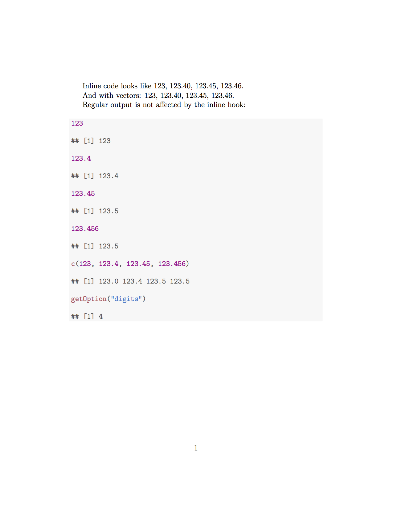
After seeing a StackOverflow answer by Josh O’Brien, I realized that the default inline_hook function for knitr could be easily modified to use the sprintf() command instead of round(). The minute change will forcibly output all manuscript values to 2 decimal places. Below, we see the default behavior for knitr when processing inline R expressions:

knitr’s Default Hook
1
2
library(knitr)
knit_hooks$get("inline")
knitr’s Default Hook
1
2
3
4
5
6
function (x)
{
    if (is.numeric(x))
        x = round(x, getOption("digits"))
    paste(as.character(x), collapse = ", ")
}

Note: My original code for this post used the format() command. Winston Chang pointed out that this could lead to unreliable output and tweaked the code to use sprintf(). The credit for the more efficient function below goes to him. Below, we add out improved inline_hook to the preamble of our knitr document:

Improving the inline_hook
1
2
3
4
5
6
7
8
9
10
11
12
13
14
15
<<>>=
library(knitr)
inline_hook <- function (x) {
  if (is.numeric(x)) {
    # ifelse does a vectorized comparison
    # If integer, print without decimal; otherwise print two places
    res <- ifelse(x == round(x),
      sprintf("%d", x),
      sprintf("%.2f", x)
    )
    paste(res, collapse = ", ")
  }
}
knit_hooks$set(inline = inline_hook)
@

Working Example

Let’s put it all together! The following is a working example of the the suggested knitr inline_hook function, which should give more reliable output by rounding inline values to 2 decimal places.

Winston’s Example
1
2
3
4
5
6
7
8
9
10
11
12
13
14
15
16
17
18
19
20
21
22
23
24
25
26
27
28
29
30
31
32
33
34
35
36
37
38
\documentclass[12pt]{article}
\begin{document}

<<load, include=FALSE, echo=FALSE>>=
library(knitr)

inline_hook <- function (x) {
  if (is.numeric(x)) {
    # ifelse does a vectorized comparison
    # If integer, print without decimal; otherwise print two places
    res <- ifelse(x == round(x),
      sprintf("%d", x),
      sprintf("%.2f", x)
    )
    paste(res, collapse = ", ")
  }
}

knit_hooks$set(inline = inline_hook)
@

Inline code looks like \Sexpr{123}, \Sexpr{123.4}, \Sexpr{123.45}, \Sexpr{123.456}.

And with vectors: \Sexpr{c(123, 123.4, 123.45, 123.456)}.

Regular output is not affected by the inline hook:

<<>>=
123
123.4
123.45
123.456

c(123, 123.4, 123.45, 123.456)

getOption('digits')
@
\end{document}

Comments