I’ve cross-posted this at the SAPA Project’s blog.
Item Response Theory can be used to evaluate the effectiveness of exams given to students. One distinguishing feature from other paradigms is that it does not assume that every question is equally difficult (or that the difficulty is tied to what the researcher said). In this way, it is an empirical investigation into the effectiveness of a given exam and can help the researcher 1) eliminate bad or problematic items and 2) judge whether the test was too difficult or the students simply didn’t study.
In the following tutorial, we’ll use R (R Core Team, 2013) along with the psych package (Revelle, W., 2013) to look at a hypothetical exam.
Before we get started, remember that R is a programming language. In the examples below, I perform operations on data using functions like cor and read.csv. We can also save the output as objects using the assignment arrow, <-. It’s a bit different from a point-and-click program like SPSS, but you don’t need to know how to program to analyze exams and questions using IRT!
First, load the the psych package. Next, load the students’ grades into R using read.csv() from the psych package.
1 2 3 4 | |
Notice that we are using item-level grades, where each row is a given student and each cell is the number of points received on that question. In my example, V1, V2, etc. correspond to exam questions. Your matrix or data frame should look like this:
1
| |
1 2 3 4 5 6 7 8 9 10 11 12 13 14 | |
Next, compute the polychoric correlations on the raw grades (not including the Total column). By using polychoric correlations, we estimate the normal distribution of latent content knowledge, which can be underestimated if Pearson correlations are instead used on polytomous items (see Lee, Poon & Bentler, 1995).
1 2 | |
Now that we have the polychoric correlations, we can run irt.fa() on the dataset to see the item difficulties and information.
1 2 3 4 | |
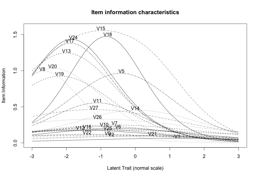
Thus, we have some great items that have a lot of information about students of average and low content knowledge (e.g., V24, V17, V18), but not enough to distinguish the high-knowledge students. In redesigning an exam for next semester or year, we might save the best performing questions while trying to rewrite the existing questions or trying new questions.
Next, let’s see what how well the test did overall at distinguishing students:
1
| |
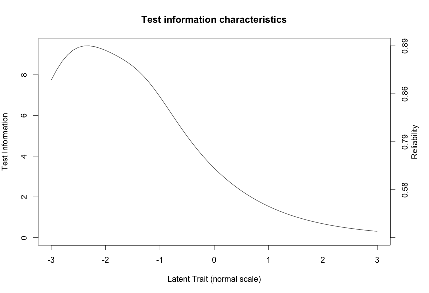
The second plot shows the test performance. We have great reliability for distinguishing who didn’t study (lowers end of our latent trait), but overall the test may have been too easy (opposite of my prediction). It’s important that the test is not too difficult to discourage students, but the graph above suggests that we had very low information at how students that studied were different from eachother. This is again reflected by the histogram plotted in the next section, where high scoring students seem to cluster together.
Rescaling the test
While many students in our hypothetical dataset did very well on the exam, instructors may
need to rescale their exam so that the mean grade is an 85% or 87.5%. Using the scale() function (see also rescale() in psych package), we
can ensure that the rank-order distribution of the students is preserved (allowing us to distinguish
those who studied well from those who didn’t), while scaling the sample distribution to fit in with other classes in your department.
Currently, our scores are in cumulative raw points. Notice that we divide the Total points column by 91 to convert the histogram into grade percentages. Let’s plot a histogram to see the distribution of scores.
1 2 3 4 5 | |
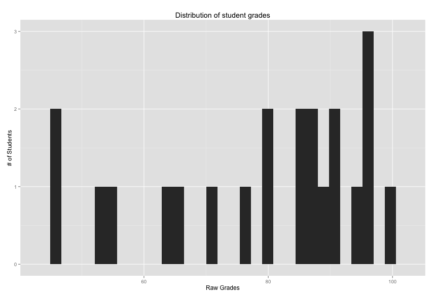
The distribution has a mean 71.68 percent and a standard deviation of 15.54. Given grade inflation, it may look like your students are doing poorly when in fact the distribution is similiar to other courses being taught. Next, we can rescale the grades, creating a mean of 87.5 and a standard deviation of 7.5. These numbers are arbitrary so use your best judgement.
1 2 3 | |
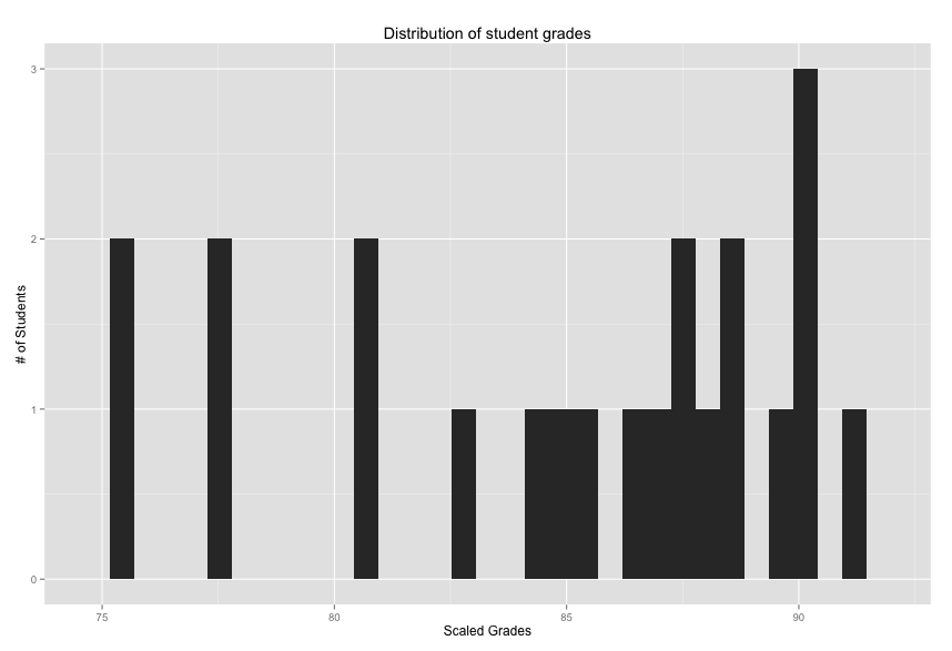
The second distribution may be preferred, depending on your needs. With the raw distribution, we would have had 45% of the students receiving grades below a C-, assuming a normal distribution (for the curious, R can calculate these probabilites using the pnorm function: pnorm(q=70,mean=71.68,sd=15.54)). Now, 0.9% of students would fall below the 70% cutoff. Again, my mean and standard deviation chosen in the above example are arbitrary.
References
Lee, S. Y., Poon, W. Y., & Bentler, P. M. (1995). A two‐stage estimation of structural equation models with continuous and polytomous variables. British Journal of Mathematical and Statistical Psychology, 48(2), 339-358.
R Core Team (2013). R: A language and environment for statistical computing. R Foundation for Statistical Computing, Vienna, Austria. http://www.R-project.org/.
Revelle, W. (2013). psych: Procedures for Personality and Psychological Research. Northwestern University, Evanston, Illinois, USA. http://CRAN.R-project.org/package=psych. Version = 1.3.10.