Overview

When I began using R, like most researchers I kept all my data in some combination of R’s native data.frame format or a CSV file that my analysis would continually read. However, as I began to analyze big datasets at the SAPA Project and at Insight, I realized that there is a lot of value to instead keeping your data in a MySQL database and streaming it into R when necessary. This post will briefly outline a few advantages of using a database to store data and run through a basic example of using R to transfer data to MySQL.

Memory Efficiency

Relational databases, such as MySQL, organize data into tables (like a spreadsheet) and can link values in tables to each other. Generally speaking, they are better at handling large datasets and are more efficient at storing and accessing data than CSVs due to compression and indexing. The data stay in the MySQL database until accessed via a query, which is different than how R approaches data.frames and CSVs. When accessing data stored in a data.frame or CSV file in R, the data must all fit in memory. However, this becomes a problem if when using a large dataset or if you’re cursed with an older computer with <= 4GB of RAM. In these cases, every time you load your dataset or do a memory-intensive operation (e.g., polychoric correlations) your computer will slow to a painful crawl as your hard drives grind while your operating system switches to using virtual memory or swap space, rather than RAM. You could get around this by using random sampling to create a smaller subset (or multiple subsets if you want to bootstrap), but you can also use this technique on a SQL database. The advantage is that SQL databases only load the data you’re working with into your local machine’s RAM when you SELECT the data you need - leaving plenty of memory for the actual analysis.

Safety and Security

Two additional reasons I prefer SQL databases are safety and security. Services such as Amazon’s RDS (i.e., Relational Database Service) offer frequent backups and easy replication across instances. If the local machine dies, the data are safe and uncorrupted. If I were storing data in an .Rdata file, I’d have to rely on my OS (e.g., Time Machine) or a cloud-based storage solution (e.g., Dropbox or CrashPlan) to backup my data. Worse, if I were storing my data in an Excel database and Excel crashed, I may risk losing years of progress.

Using MySQL, I can give a collaborator access to only needed portions of the data by locking down their SQL user to certain tables and operations. By limiting access, we limit risk of corruption and overwriting years of progress.

Scalable as the need grows

Last, I find databases such as MySQL to be more scalable due to cloud computing. In the case of using Amazon’s RDS, you can buy as much storage or bandwidth as you need to complete your analysis, dissertation, or build your web app. If I need multiple nodes or machines to analyze the data, I don’t need to keep a copy of the data on each machine. I simply pass the SQL authentication parameters to each machine and the data is accessed from a central location.

So let’s begin by setting up a Free-Tier RDS service on Amazon and then move some data from R to the RDS database.

Setting up an RDS Instance

Amazon currently offers a Free Tier for their RDS storage. It offers:

• Enough hours to run a DB Instance continuously each month,
• 20 GB of database storage,
• 10 million I/O operations, and
• automated database backups.

To setup an RDS instance:

1. Sign into the AWS Management Console.
2. Select ‘RDS’ under the ‘Database’ group.
3. Click ‘Launch DB Instance’.
4. Select ‘MySQL’ for the database engine.
5. Select ‘No’ when asked if you intend to use the database for production purposes. Accidentally selecting ‘Yes’ could result in hefty fees.
6. For ‘Instance Class’, select ‘db.t1.micro’, ‘No’ for ‘Multi-AZ Deployment’, and 20 GB for ‘Allocated Storage’.
7. Click ‘Next’ and launch your RDS instance.

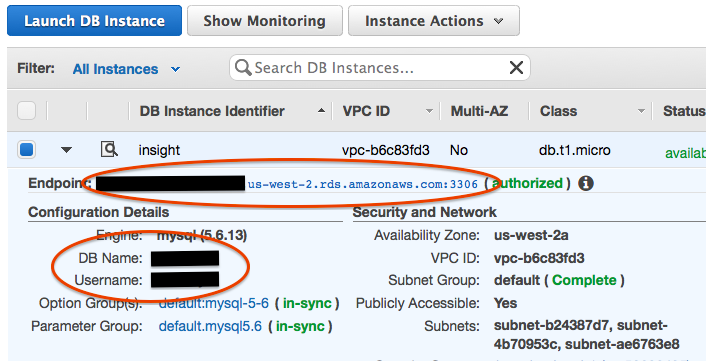
At this point, you should have a blank RDS database with a master username and password combination. Be sure to test that you can connect - I suggest using Sequel Pro. If you can’t connect, you may need to open up port 3306 in your EC2 Security Group.

Click on your new RDS Instance to get the hostname to connect to and note the database name:

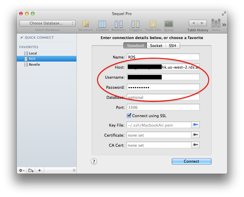
Fire up Sequel Pro and test out your new database. If you want to connect using SSL, you’ll need the SSH key you generated when you first created your EC2 instance (not covered here).

Installing the RMySQL package

Previously, I found installing RMySQL to be very difficult when I was using MacPorts. However, having switched to Homebrew on my new machine, RMySQL found all the MySQL headers and libraries as Homebrew uses the /usr/local directory to store your software, which is already in your shell $PATH.

Before compiling RMySQL, first compile MySQL using Homebrew:

1
2
3
4
5

# If you haven't already, install Homebrew:
# ruby -e "$(curl -fsSL https://raw.github.com/Homebrew/homebrew/go/install)"

# Install MySQL
brew install mysql

1
2
3
4
5
6
7
8
9
10
11
12
13
14
15
16
17
18

==> Downloading https://downloads.sf.net/project/machomebrew/Bottles/mysql-5.6.1
Already downloaded: /Library/Caches/Homebrew/mysql-5.6.19.mavericks.bottle.tar.gz
==> Pouring mysql-5.6.19.mavericks.bottle.tar.gz
==> Caveats
A "/etc/my.cnf" from another install may interfere with a Homebrew-built
server starting up correctly.

To connect:
    mysql -uroot

To have launchd start mysql at login:
    ln -sfv /usr/local/opt/mysql/*.plist ~/Library/LaunchAgents
Then to load mysql now:
    launchctl load ~/Library/LaunchAgents/homebrew.mxcl.mysql.plist
Or, if you don't want/need launchctl, you can just run:
    mysql.server start
==> Summary
🍺  /usr/local/Cellar/mysql/5.6.19: 9536 files, 338M

Next, compile RMySQL from source:

1

install.packages('RMySQL', type = 'source')

1
2
3
4
5
6
7
8
9
10
11
12
13
14
15
16
17
18
19
20
21
22
23
24
25
26
27
28
29
30
31
32
33
34
35
36
37
38
39
40
41
42
43
44
45
46
47
48
49
50
51
52
53
54
55
56
57
58

trying URL 'http://cran.rstudio.com/src/contrib/RMySQL_0.9-3.tar.gz'
Content type 'application/x-gzip' length 165363 bytes (161 Kb)
opened URL
==================================================
downloaded 161 Kb

* installing *source* package ‘RMySQL’ ...
** package ‘RMySQL’ successfully unpacked and MD5 sums checked
checking for gcc... gcc
checking for C compiler default output file name... a.out
checking whether the C compiler works... yes
checking whether we are cross compiling... no
checking for suffix of executables...
checking for suffix of object files... o
checking whether we are using the GNU C compiler... yes
checking whether gcc accepts -g... yes
checking for gcc option to accept ANSI C... none needed
checking how to run the C preprocessor... gcc -E
checking for compress in -lz... yes
checking for getopt_long in -lc... yes
checking for mysql_init in -lmysqlclient... yes
checking for egrep... grep -E
checking for ANSI C header files...
rm: conftest.dSYM: is a directory
rm: conftest.dSYM: is a directory
yes
checking for sys/types.h... yes
checking for sys/stat.h... yes
checking for stdlib.h... yes
checking for string.h... yes
checking for memory.h... yes
checking for strings.h... yes
checking for inttypes.h... yes
checking for stdint.h... yes
checking for unistd.h... yes
checking mysql.h usability... no
checking mysql.h presence... no
checking for mysql.h... no
checking /usr/local/include/mysql/mysql.h usability... yes
checking /usr/local/include/mysql/mysql.h presence... yes
checking for /usr/local/include/mysql/mysql.h... yes
configure: creating ./config.status
config.status: creating src/Makevars
** libs
clang -I/Library/Frameworks/R.framework/Resources/include -DNDEBUG -I/usr/local/include/mysql -I/usr/local/include -I/usr/local/include/freetype2 -I/opt/X11/include    -fPIC  -Wall -mtune=core2 -g -O2  -c RS-DBI.c -o RS-DBI.o
clang -I/Library/Frameworks/R.framework/Resources/include -DNDEBUG -I/usr/local/include/mysql -I/usr/local/include -I/usr/local/include/freetype2 -I/opt/X11/include    -fPIC  -Wall -mtune=core2 -g -O2  -c RS-MySQL.c -o RS-MySQL.o
clang -dynamiclib -Wl,-headerpad_max_install_names -undefined dynamic_lookup -single_module -multiply_defined suppress -L/usr/local/lib -o RMySQL.so RS-DBI.o RS-MySQL.o -lmysqlclient -lz -F/Library/Frameworks/R.framework/.. -framework R -Wl,-framework -Wl,CoreFoundation
installing to /Library/Frameworks/R.framework/Versions/3.1/Resources/library/RMySQL/libs
** R
** inst
** preparing package for lazy loading
Creating a generic function for ‘format’ from package ‘base’ in package ‘RMySQL’
Creating a generic function for ‘print’ from package ‘base’ in package ‘RMySQL’
** help
*** installing help indices
** building package indices
** testing if installed package can be loaded
* DONE (RMySQL)

Transferring Existing Data to/from MySQL

Having a database is useless unless we can easily convert our existing data.frames into MySQL tables. Let’s try this using the Thurstone dataset from the Revelle’s psych package:

1
2
3
4
5
6
7
8

library(RMySQL)
library(psych)
con <- dbConnect(MySQL(),
    user = 'RDSUser',
    password = 'YourPass',
    host = 'RDS Host',
    dbname='YourDB')
dbWriteTable(conn = con, name = 'Test', value = as.data.frame(Thurstone))

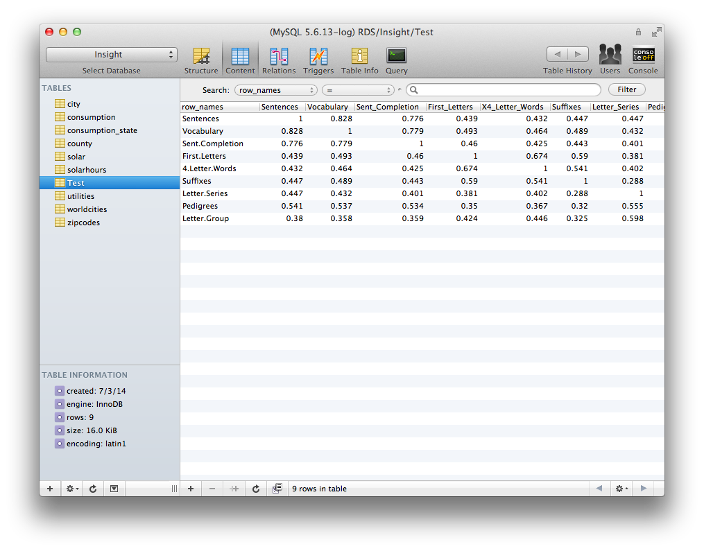
There! Now we have transferred our data.frame to our SQL database.

Similarly, if you want to read data from MySQL to R, we can use the dbReadTable() function, which returns a data.frame object. You can keep your data in MySQL and stream portions into R for specific analyses. Since dbReadTable outputs a data.frame, we can use this command in place of a data.frame.

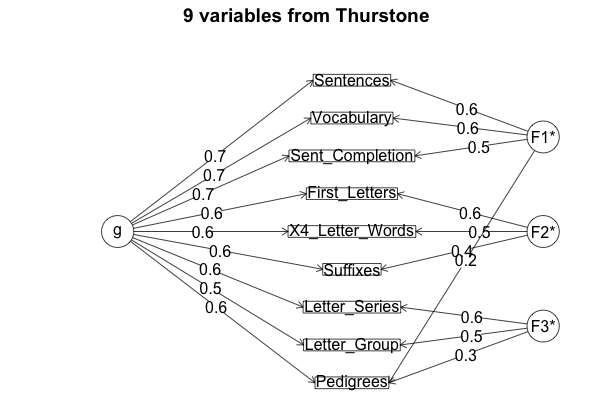
Let’s run an omega() factor analysis on the Thurstone table:

1

omega(dbReadTable(conn = con,name = 'Test'), title = "9 variables from Thurstone")

1
2
3
4
5
6
7
8
9
10
11
12
13
14
15
16
17
18
19
20
21
22
23
24
25
26
27
28
29
30
31
32
33
34
35
36
37
38
39
40
41
42
43
44
45
46
47
48
49
50
51
52
53

Loading required package: MASS
Loading required package: GPArotation
Loading required package: parallel
9 variables from Thurstone
Call: omega(m = dbReadTable(conn = con, name = "Test"), title = "9 variables from Thurstone")
Alpha:                 0.89
G.6:                   0.91
Omega Hierarchical:    0.74
Omega H asymptotic:    0.79
Omega Total            0.93

Schmid Leiman Factor loadings greater than  0.2
                   g   F1*   F2*   F3*   h2   u2   p2
Sentences       0.71  0.57             0.82 0.18 0.61
Vocabulary      0.73  0.55             0.84 0.16 0.63
Sent_Completion 0.68  0.52             0.73 0.27 0.63
First_Letters   0.65        0.56       0.73 0.27 0.57
X4_Letter_Words 0.62        0.49       0.63 0.37 0.61
Suffixes        0.56        0.41       0.50 0.50 0.63
Letter_Series   0.59              0.61 0.72 0.28 0.48
Pedigrees       0.58  0.23        0.34 0.50 0.50 0.66
Letter_Group    0.54              0.46 0.53 0.47 0.56

With eigenvalues of:
   g  F1*  F2*  F3*
3.58 0.96 0.74 0.71

general/max  3.71   max/min =   1.35
mean percent general =  0.6    with sd =  0.05 and cv of  0.09
Explained Common Variance of the general factor =  0.6

The degrees of freedom are 12  and the fit is  0.01

The root mean square of the residuals is  0.01
The df corrected root mean square of the residuals is  0.01

Compare this with the adequacy of just a general factor and no group factors
The degrees of freedom for just the general factor are 27  and the fit is  1.48

The root mean square of the residuals is  0.14
The df corrected root mean square of the residuals is  0.16

Measures of factor score adequacy
                                                 g  F1*  F2*  F3*
Correlation of scores with factors            0.86 0.73 0.72 0.75
Multiple R square of scores with factors      0.74 0.54 0.52 0.56
Minimum correlation of factor score estimates 0.49 0.08 0.03 0.11

 Total, General and Subset omega for each subset
                                                 g  F1*  F2*  F3*
Omega total for total scores and subscales    0.93 0.92 0.83 0.79
Omega general for total scores and subscales  0.74 0.58 0.50 0.47
Omega group for total scores and subscales    0.16 0.35 0.32 0.32

In other analyses, you may only need a fraction of the MySQL table. In these cases, we’d want to use the dbGetQuery() command and issue a MySQL statement to SELECT and aggregate the information. Let’s get a vector of Sentences correlations that are greater than 0.5:

1

dbGetQuery(conn = con, statement = "SELECT Sentences FROM Test WHERE Sentences > 0.5;")

1
2
3
4
5

  Sentences
1     1.000
2     0.828
3     0.776
4     0.541

Safely storing credentials

It’s important to note that in the above example, although I passed the user and password parameters within my dbConnect() function, you would never want to do this in production code that you were sharing. It’s far better to store the credentials a text file where dbConnect(MySQL()) will look when you don’t pass any credentials:

1
2
3
4

user = youruser
password = yourpassword
host = yourhouse
dbname = yourdb

Useful Packages for Fast DB Operations

Ideally, we want to have one set of analysis code that is agnostic to how the data are stored. I suggest looking into Hadley Wickham’s new dplyr package (Github). dplyr is able to filter, sort, group, and summarize data quickly whether it is stored in a data.frame, data.table, or database. Database operations may not always be as fast as a data.table operation, but again, the advantage is that you don’t need to feed all of your data into memory.

Hadley provides a few vignettes for getting getting started with dplyr:

1
2

vignette("introduction", package = "dplyr")
vignette("databases", package = "dplyr")